CPSC 352 -- Artificial Intelligence
Notes: Machine Learning: Neural Networks
Introduction
In this lecture we consider the basics of machine learning in neural networks.
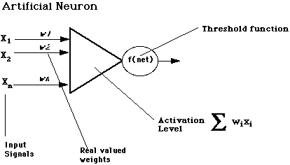
An Artificial Neuron
Connectionist Learning
Hebbian Learning (1949):
Repeated stimulation between two or more
neurons strengthens the connection weights among those neurons. One problem
with this model is it had no way to model inhibition between neurons.
Perceptron Learning (1958):
A perceptron is a single-layer network that calculates a
linear combination of its inputs and outputs a 1 if the result is greater
than some threshold and a -1 if it is not:
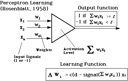
Supervised Perceptron Learning
- c : learning-rate parameter
- d: desired output value
- signal() is the perceptron's actual output value, which is always +1 or -1
- cases
- d - signal = 0 ==> do nothing
- d - signal = +2 ==> increment wi by 2cxi
- d - signal = -2==> decrement wi by 2cxi
By repeatedly adjusting weights in this fashion for an entire set of
training data, the perceptron will minimize the average error
over the entire set.
Minsky and Papert (1969) showed that if there is a set of weights that
give the correct output for an entire training set, a perceptron will learn it.
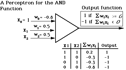
Example: Perceptrons can learn models for the following
primitive boolean functions: AND, OR, NOT, NAND, NOR. Here's an
example for AND:
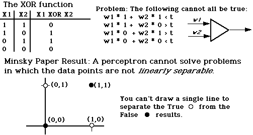
Limitations of Perceptrons
Minsky and Papert (1969) showed that perceptrons could not model the exclusive-or
function, because its outputs are not linearly separable. Two classes of
outputs are linearly separable if and only if you can draw a straight line in
two dimensions that separates one classification from another.
The Delta Rule (Rumelhart, 1986)
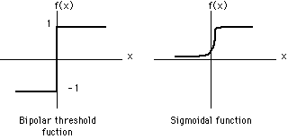
The perceptron activation function is a hard-limiting threshold function.
A more general neural network uses a continuous activation function. One popular
function is the sigmoidal (s-shaped) function, such as the logistic function:
f(net) = 1/(1 + e-L*net)
where L is lambda, a
parameter for "squashing" the function and net is the output or
sum of the weights.
The delta rule is a learning rule for a network with a
continuous (and therefore differentiable) activation function. It attempts
to minimize the cumulative error over a data set as a function of
the weights in the network:
Delta(wji) = c(di - Oi)f'(neti)xj
where c is the learning rate, di and Oi are the
desired and actual outputs for the ith node, and f'(net) is the derivative of the activation
function for the ith node, and xj is the jth input to the ith node.
Key Point: The delta rule is tries to minimize the slope of the cumulative
error in a particular region of the network's output function. This makes is susceptible
to local minima.
Back propagation Learning for Multilayer Networks
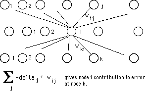
Back propagation starts at the output layer and propagates the error backwards
through the network. The learning rule is often called the generalized delta rule.
Back propagation activation function is the logistic function:
f(net) = 1/(1 + e-L*net)
The logistic function is useful for assigning error to the hidden layers in a multi-layer
network because:
- It is continuous and has a derivative everywhere.
- It is sigmoidal.
- The derivative is greatest where the function is steepest. This
assigns the most error to nodes whose activation is least certain.
The formulas for computing the adjustments of the kth weight of the ith node:
Delta(wik) = -c(di - Oi) * Oi(1 - Oi)xik
for nodes on the output layer
Delta(wik) = -c * Oi(1 - Oi)Sum(-deltaj * wij)xik
for nodes on the hidden layers.
NETtalk System (Sejnowski and Rosenberg, 1987)
Nettalk is a neural network, developed in 1987, that learns to pronounce
English text. It learns to associate phonemes with string of text.
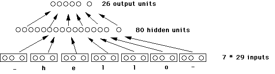
Properties of NETtalk
- Learned to pronounce English text.
- Inputs: String of text, e.g. "I say hello to you" (7 letter window)
- Input Unit: 29 units, one for each letter and 3 for punctuation and spaces
- Outputs: Phonemes (26 different ones)
- Hidden Elements: 80 (These units learn the pronounciation rules)
- Connections: 18,629
- Learning rule: back propagation
- Interesting Properties
- Performance improves with training but at a slower rate.
- Graceful degradation
- Relearning was highly efficient
NETtalk Comparison with ID3 (Shavlik, 1991)
- Both ID3 and NETtalk were able to pronounce 60% after 500 training examples
- ID3 required 1 pass through the training data
- NETtalk was allowed 100 passes through the 500 training data
Using Encog Java Neural Network Framework
Homework Exercise: Using the links below, download the
Encog Framework into
a directory on your Linux account. Then perform the exercises.
Downloads Download and unzip each of the following Encog
packages from the Encog Download Site:
- encog-workbench-3.0.1-release.zip
- encog-examples-3.0.1-release.zip
- encog-core-3.0.1-release.zip
Exercises
- Take a look at
the Getting
Started Documentation.
- Command Line Exercise: Do the Encog
Java XORHelloWorld
example. Try working through the ANT version. On my system, this is the Java
command you need to run from within the .../encog-examples-3.0.1/lib:
java -cp encog-core-3.0.1-SNAPSHOT.jar:examples.jar org.encog.examples.neural.xor.XORHelloWorld
- GUI Exercise: Do
the Workbench
Classification Example.