Introduction

• Is the search guaranteed to find a solution?
• Will the search always terminate (or will it loop endlessly)?
• Will the solution, if found, be optimal?
• How complex is the search process?
• How can the complexity of the search be reduced?
• How can the search be designed to use a representation language?

A Bit of Graph Theory

Bridges of Konigsberg

The city of Konigsberg occupied both banks and two islands of a river. The islands and the riverbanks were connected by seven bridges, as shown in the following graph. Is there a path through the city that crosses each bridge exactly once?

Euler's Proof

   connect(i1, i2, b1).			connect(i2, i1, b1).
   connect(rb1, i1, b2).		connect(i1, rb1, b2).
   connect(rb1, i1, b3).		connect(i1, rb1, b3).
   connect(rb1, i2, b4).		connect(i2, rb1, b4).
   connect(rb2, i1, b5).		connect(i1, rb2, b5).
   connect(rb2, i1, b6).		connect(i1, rb2, b6).
   connect(rb2, i2, b7).		connect(i2, rb2, b7).

This way does not lend itself to Euler's proof. This shows the important of knowledge representation. One representation (graph) leads to a simple proof. The other does not.

Graph Definitions

• A graph consists of:

  • A set of nodes N₁, N₂, N₃, ..., N₃, ...

  • A set of arcs that connect pairs of nodes. So arcs can be described as ordered pairs (N₁, N₂).

• An directed graph has an indicated direction for traversing each arc.

  

• If a directed arc connects N_j and N_k, the N_j is called the parent of N_k, and N_k is called the child of N_j. If the graph also contains an arc (N_j, N_l), then N_k and N_l are called siblings

• A rooted graph has a unique node N_s from which all paths originate.

• A tip or leaf is a node that has no children.

• An ordered sequence of nodes [N₁, N₂, N₃, ..., N_n], where each N_i and N_i+1 in the sequence represents an arc, is called a path of length n in the graph.

• On a path in a rooted graph, a state is said to be an ancestor of all states positioned after it (to its right) and a descendant of all states before it (to its left).

• A path that contains any state more than once is said to contain a cycle or loop.

• A tree is a graph in which there is a unique path between every pair of nodes. The edges in a rooted tree are directed away from the root. Each node in a rooted tree has a unique parent.

  

• Two states in a graph are said to be connected if a path exists that includes both.

State Space Representation of Problems

A state space is represented by a four-tuple [N, A, S, GD]

• N is a set of nodes or states of the graph. These correspond to the states in a problem-solving process.

• A is the set of arcs between the nodes. These correspond to the steps or moves in a problem-solving process.

• S , a nonempty subset of N , contains the start state(s) of the problem.

• GD , a nonempty subset of N , contains the goal state(s) of the problem. The states in GD are described using either:
  1. A measurable property of the states encountered in the search.

  2. A property of the path developed in the search.

Example: Traveling Salesman Problem

Starting at A, find the shortest path through all the cities, visiting each city exactly once and returning to A.

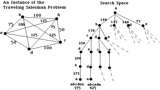
Reducing Search Complexity: For N cities, a brute-force solution to the traveling salesman problem takes N! time. There are ways to reduce this complexity:

• Branch and Bound Algorithm: Generate one path at a time, keeping track of the best circuit so far. Use the best circuit so far as a bound on future branches of the search. This reduces the complexity to 1.26^N.

• Nearest Neighbor Heuristic: At each stage of the circuit, go to the nearest unvisited city. This strategy reduces the complexity to N, so it is highly efficient, but it is not guaranteed to find the shortest path, as the following example shows:

  

In-class Exercise

Missionaries and Cannibals Problem: Give the state-space graph for the missionaries and cannibals problem. There are 3 missionaries and 3 cannibals on the side of a river which must be crossed in a boat that can hold at most 2 people at once. If the missionaries ever outnumber the cannibals on one or the other bank, they will convert the cannibals. Find an crossing strategy that gets the whole party to the opposite bank without losing any cannibals. Represent the start state as follows: [[m m m c c c] []]. Don't show transitions to duplicate states.

Data-Driven and Goal-Driven Search

In data-driven search, sometimes called forward chaining, the problem solver begins with the given facts and a set of legal moves or rules for changing the state. Search proceeds by applying rules to facts to produce new facts. This process continues until (hopefully) it generates a path that satisfies the gaol condition.

In goal-driven search, sometimes called backward chaining, the problem solver begins with the goal to be solved, then finds rules or moves that could be used to generate this goal and determine what conditions must be true to use them. These conditions become the new goals, subgoals, for the search. This process continues, working backward through successive subgoals, until (hopefully) a path is generated that leads back to the facts of the problem.

Data-driven and goal-driven are relative concepts. They depend on how one chooses to represent the search space.

Example of Data Driven Search

   (A ^ B) -> (C ^ D)
   A             
   B              / Therefore, D

   1.  (A ^ B) -> (C ^ D)
   2.  A             
   3.  B              / Therefore, D
   4.  A ^ B          From 2, 3 by Conjunction
   5.  C ^ D          From 1, 4 by Modus ponens
   6.  D ^ C          From 5 by Commutation
   7.  D              From 6 by Simplification  

Example of Goal Driven Search

   (A ^ B) -> (C ^ D)
   A             
   B              / Therefore, D

   1.  D           
   2.  D ^ C              This subgoal can produce 1 by Simplification
   3.  C ^ D              This subgoal can produce 2 by Commutation
   4.  A ^ B              This subgoal 
   5.  (A ^ B) -> (C ^ D)   and this premise can produce 3 by Modus Ponens
   6.  A                  This premise
   7.  B                    and this premise can produce 4 by Conjunction

Goal-Driven and Data-Driven Strategies

Goal-driven search uses knowledge of the goal to guide the search. Use goal-driven search if;

• A goal or hypothesis is given in the problem or can easily be formulated. (Theorem proving; medical diagnosis; mechanical diagnosis)

• There are a large number of rules that match the facts of the problem and would thus produce an increasing number of conclusions or goals. (inefficient)

• Problem data are not given but must be acquired by the problem solver. (e.g., medical tests determined by possible diagnosis)

• All or most of the data are given in the initial problem statement.

• There are a large number of potential goals, but there are only a few ways to use the facts and the given information of a particular problem.

• It is difficult to form a goal or hypothesis.

In-class Exercise

Car Won't Start: Sketch the state space graph for the problem of diagnosing why your car won't start. Discuss the pros and cons of using a data-driven versus a goal-driven search strategy for this problem.

The first problem you have to solve is what the states in the graph represent. Let the states represent partial knowledge about the cause of the problem, with the goal being complete knowledge of the cause. So the goals are states such as: out-of-gas, dead-battery, and so on. Let the start state be zero knowledge. (See page 43.)

Question: Is this the only way to represent this problem?

Backtracking Search Algorithm

The backtrack algorithm uses three lists plus one variable:

• SL, the state list, lists the states in the current path being tried. If a goal is found, SL contains the ordered list of states on the solution path.

• NSL, the new state list, contains nodes awaiting evaluation -- i.e., nodes whose descendants have not yet been generated and searched.

• DE, dead ends, lists states whose descendants have failed to contain a goal node. If these states are encountered again, they will be immediately eliminated from consideration.

• CS, the current state.

The Backtrack Algorithm

  SL := [Start]; NSL := [Start]; DE := []; CS := Start;  // Initialize
  while NSL != [] {
      if CS = goal (or meets goal description)
          return SL;                                     // Success
      if CS has no children (except those on DE, SL, or NSL) {
          while SL != [] and CS = first element of SL {
              add CS to DE;                              // Dead End
              remove first element of SL;                // Backtrack
              remove first element of NSL;
              CS := first element of NSL;
          }
          add CS to SL;
      } else {
          place children of CS (except those on DE, SL, NSL) onto NSL;
          CS := first element of NSL;
          add CS to SL;
      }
  }
  return FAIL;                                           // Failure

A Trace of Backtrack Algorithm

    AFTER     CS    SL            NSL               DE
  ITERATION
     0        A     [A]           [A]               []
     1        B     [B A]         [B C D A]         []
     2        E     [E B A]       [E F B C D A]     []
     3        H     [H E B A]     [H I E F B C D A] []
     4        I     [I E B A]     [I E F B C D A]   [H]
     5        F     [F B A]       [F B C D A]       [E I H]
     6        J     [J F B A]     [J F B C D A]     [E I H]
     7        C     [C A]         [C D A]           [B F J E I H]
     8        G     [G C A]       [G C D A]         [B F J E I H]

Depth-First and Breadth-First Search

In addition to the search direction (data- or goal-driven) a search is determined by the order in which the nodes are examined: breadth first or depth first.

Consider the following graph:

Depth First Search examines the nodes in the following order:

  A, B, E, K, S, L, T, F, M, C, G, N, H, O, P, U, D, I, Q, J, R

Breadth First Search examines the nodes in the following order:

  A, B, C, D, E, F, G, H, I, J, K, L, M, N, O, P, Q, R, S, T, U

Breadth First Search Algorithm

In breadth-first search, when a state is examined, all of its siblings are examined before any of its children. The space is searched level-by-level, proceeding all the way across one level before going down to the next level.

In the following algorithm the open list is like NSL in the backtrack algorithm. It contains states that have been generated but whose children have not been examined. The closed list is the union of the DE and SL. It contains states that have already been examined.

  open := [Start];                                       // Initialize
  closed := [];
  while open != [] {                                     // While states remain
      remove the leftmost state from open, call it X;
      if X is a goal
          return success;                                // Success
      else {
          generate children of X;
          put X on closed;
          eliminate children of X on open or closed;     // Avoid loops
          put remaining children on RIGHT END of open;    // Queue
      }
  }
  return failure;                                        // Failure

Note that, unlike backtrack, this algorithm does not store the solution path. If you want the solution path, you should retain ancestor information on the closed list. For example, an ordered pair, (child, parent), can be kept on the closed and open lists. This allows the solution path to be constructed from the closed list.

A Trace of Breadth-first Algorithm: Search for U

    AFTER     open                closed
  ITERATION
     0        [A]                 [] 
     1        [B C D]             [A]        
     2        [C D E F]           [B A] 
     3        [D E F G H]         [C B A]
     4        [E F G H I J]       [D C B A]
     5        [F G H I J K L]     [E D C B A]
     6        [G H I J K L M]     [F E D C B A]     
     7        [H I J K L M N]     [G F E D C B A]
     8        and so on until U is found or open = []

Optimality: Breadth-first search is guaranteed to find the shortest path to the goal, if a path to the goal exists.

Depth First Search Algorithm

In depth-first search, when a state is examined, all of its children and their descendants are examined before any of its siblings.

  open := [Start];                                       // Initialize
  closed := [];
  while open != [] {                                     // While states remain
      remove the leftmost state from open, call it X;
      if X is a goal
          return success;                                // Success
      else {
          generate children of X;
          put X on closed;
          eliminate children of X on open or closed;     // Avoid loops
          put remaining children on LEFT END of open;     // Stack
      }
  }
  return failure;                                        // Failure

A Trace of Depth-first Algorithm: Search for U

    AFTER     open                closed
  ITERATION
     0        [A]                 [] 
     1        [B C D]             [A]        
     2        [E F C D]           [B A] 
     3        [K L F C D]         [E B A]
     4        [S L F C D]         [K E B A]
     5        [L F C D]           [S K E B A]
     6        [T F C D]           [L S K E B A]     
     7        [F C D]             [T L S K E B A]
     8        [M C D]             [F T L S K E B A]
     9        [C D]               [M F T L S K E B A]
     10       [G H D]             [C M F T L S K E B A]
     11        and so on until U is found or open = []

Depth First vs. Breadth First

• Breadth first is guaranteed to find the shortest path from start to goal.

• Use breadth first when it is known that a simple (short) solution exists.

• The space utilization of breadth first, measured in terms of the size of the open list, is Bⁿ where B is the branching factor -- the average number of descendants per state -- and n is the level.

• Depth first is NOT guaranteed to find the shortest path but it gets deeply into the search space.

• Depth first is more efficient for spaces with a large branching factor, because it does not have to keep all nodes at a given level on the open.

• Space utilization of depth first is linear: B * n, since at each level the open list contains the children of a single node.

• Use depth first if it is known that the solution path will be long.

• Depth first can get "lost" on a deep branch that doesn't lead to a goal.

In-class Exercise

Missionaries and Cannibals Problem: Discuss the advantages of depth-first vs. breadth-first search for this problem.

Depth First with Iterative Deepening

   Perform depth-fist with a bound of 1 level.
   If goal not found, perform depth-first with a bound of 2.
   If goal not found, perform depth-first with a bound of 3.
   . . .

So at each iteration, a complete depth-first search is performed. It is guaranteed to find the shortest path, and its space utilization at any level n is B * n.

Time Complexity

Using State Space to Represent Reasoning in Logic

State Space Search in Logic

Problems in predicate calculus, such as determining whether one expression follows from a set of assertions, can be solved using graph search. Consider this example from the propositional calculus:

And/Or Graph

An and/or graph lets us represent expressions of the form p ^ q => r.

Using the above AND/OR graph, answer each of the following questions:

• Is h true?
• Is h true if b is no longer true?
• What is the shortest path to show that X is true?
• How would you show that some proposition p is false?

And/Or Predicate Calculus Graph

Using the following AND/OR graph, where is fred?